Performance and Costs of Aggregation Features

Architecture Background

The data pipeline that Tecton manages for aggregation features consists of the following steps:

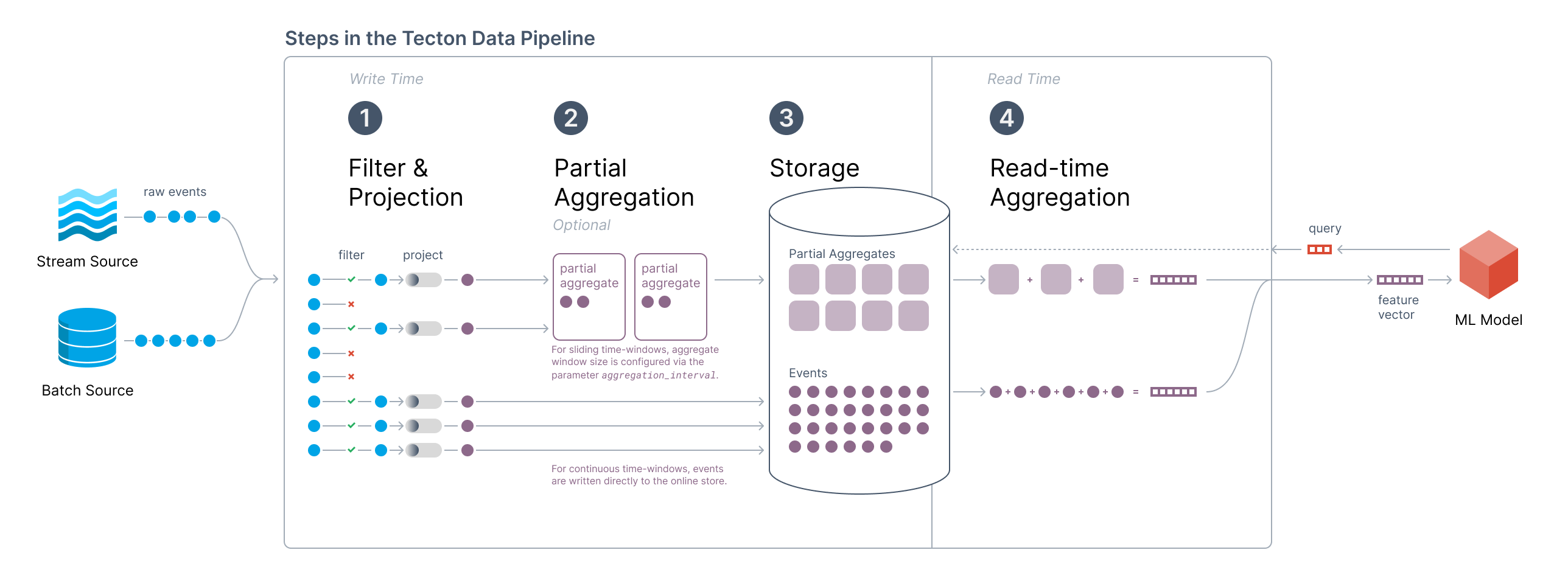
1. Filter + Projection:
   • This is the user-defined SQL / Python transformation that’s specified in a Batch or Stream Feature View.
2. Optional Partial Aggregations:
   • When Tecton aggregations with sliding windows are configured, Tecton will compute partial aggregation values for each aggregation interval time window (configured by the aggregation_interval parameter for a Feature View).
3. Online Store:
   • When using sliding windows, Tecton will write partial aggregations to the online store.
   • If instead Tecton aggregations with continuous windows are configured, then Tecton will write all projected events directly to the online store.
     • Note: Continuous windows can only be configured with Stream Feature Views.
4. Read-Time Aggregation:
   • At feature request time, Tecton will build the final feature vector by aggregating over all relevant partial aggregations or events in real-time.

note

The same behavior is true for the offline path that Tecton manages. The only difference is that the data will be stored in an offline store.

Performance at Feature Request

As a result of the read-time aggregation step mentioned above, feature retrieval latencies will vary depending on the number of rows (partial aggregations or events) being read from the online store and aggregated at the time of the request.

The factors that influence the number of rows in the online store will differ based on whether the window is sliding or continuous.

Continuous Windows

As noted in this section, when using continuous windows Tecton will write all events from the stream directly into the online store. At request time, Tecton will read all events for the requested entity in the aggregation time window and compute the final aggregation value.

As a result, the expected request-time latencies for continuous windowed aggregations will scale with the number of events per entity in the given time window.

It is important to note that the performance is only a function of the number of persisted events for the requested entity (e.g. user user_123). The read performance is not affected by materialized data for other entities.

Sliding Windows

With sliding windows, Tecton will compute partial aggregations for each entity when materializing to the online store. The size of the partial aggregations is set by the aggregation_interval parameter in the Stream Feature View.

Tecton will write 1 entry to the online store per aggregation interval for each entity with raw events in the aggregation interval window. No rows will be written for an entity with no raw events in the aggregation interval window.

At request time, Tecton will read all partial aggregations for the given entity within the feature’s aggregation time-window and compute the final aggregation value. The number of rows that will be read will be equal to the number of non-zero partial aggregations for the given entity in the max time window. This number will therefore never exceed the time_window divided by the aggregation_interval, but can often be much less depending on the distribution of raw events per entity.

Example

Let’s take a look at a quick example Stream Feature View:

@stream_feature_view(
    sources=[transactions],
    entities=[user],
    mode="spark_sql",
    aggregation_interval=timedelta(minutes=5),
    aggregations=[Aggregation(function="sum", column="amt", time_window=timedelta(days=30))],
    online=True,
    offline=True,
    feature_start_time=datetime(2021, 1, 1),
)
def user_transaction_amount_sums(transactions):
    return f"""
        SELECT user_id, timestamp, amt
        FROM {transactions}
        """

In this example, Tecton will compute 5-minute partial aggregations for each entity in a streaming job and write the values to the online store (for more information on streaming materialization, read Streaming Materialization with Spark).

At request time, if we ask Tecton to return the feature value (i.e. the 30-day transaction sum) for user_123, Tecton will read all 5-minute partial aggregations in the 30 day window for user_123 from the online store and sum them up.

In the worst case, this will be 8640 rows (30 days / 5 minutes). However, it would be extremely improbable for a user to have made transactions in every 5-minute window in the last 30 days. More commonly, we may expect to find a few dozen rows for a user.

Hence we can see why the online performance can vary greatly depending on your underlying data.

Cost Implications

Given the information outlined above, the online store cost is typically a function of:

• The amount of data stored
• The write-time QPS
• The read-time QPS

Continuous window streaming features will have the highest cost implications on the online store, because they:

• store every single projected event
• read every event at request-time

In contrast, sliding window streaming features allow you to better control costs because:

• Only partial aggregations are stored - not all projected events
• At read time, only the partial aggregations are read, which puts a strict upper bound on the amount of data that needs to be read to build the final feature vector

Of course, that cost-advantage comes at the expense of feature freshness.

Benchmarking Performance

As we can see from the sections above, online retrieval latencies for stream aggregations will depend on:

• The max time_window of the aggregations being requested
• The distribution of raw events on the stream for a given entity in a given time window
• The stream_processing_mode of the Stream Feature View (for configuring sliding vs. continuous windows)
• The aggregation_interval of the Batch or Stream Feature View (when using sliding windows)

Because data distributions vary by use case, we recommend benchmarking the online retrieval latencies for your time-window aggregations at various levels of freshness (i.e. continuous windows vs. sliding windows with varying aggregation_interval sizes). You should choose a freshness value that enables the model performance and retrieval latencies you are looking for.

tip

We suggest first testing various configurations of feature freshness in offline training to understand the impact on model performance.

Alternatives

If you need extremely fresh aggregation features over large time-windows with a high cardinality of events per entity and are unable to meet your desired online retrieval latencies, then you may consider splitting your feature into two:

• A Batch Feature View which computes a large time window at a lesser frequency (e.g. a 1 year time_window and 1 day aggregation_interval)
• A Stream Feature View which computes a smaller time window more frequently (e.g. a 1 day time_window with Continuous Stream Processing Mode)

Note that these values will still be subject to your data and should be tuned accordingly.

We recommend including these as two different features in your model and testing how it affects performance.

Impact on Cost

As compared to a single Stream Feature View, this alternative will result in more writes to the online store (due to the additional Batch Feature View) during steady-state forward fill materialization, but less writes during a backfill. This is because the Batch Feature View will only be writing 1 value per entity per aggregation_interval and the Stream Feature View will be backfilling over a smaller range.